Using Heavy Tail Optimization to Evaluate the 2023 Milliman Study Allocation

Introduction:

This paper studies the properties of Real Assets within the typical institutional portfolio. Real Assets have acted as an effective portfolio diversifier over the past 25 years. We show that the typical Pension Fund could benefit from an increased allocation to Agricultural Assets within their Real Asset allocation, which is predominantly allocated to Commercial Real Estate. In terms of constrained portfolio efficiency, the risk of the portfolio could be cut significantly, all while increasing performance by up to 42% when consideration is given to optimal weighting by way of heavy tail optimization – an improved model over mean-variance optimization. We make the case that Real Assets in general should see higher allocations in Institutional portfolios.

1. Data and Methodology:

The 2023 Milliman Public Pension Funding Study, based on the review of the top 100 largest U.S. public pension plans, describes the typical asset allocation of pension plans in the US. The main asset classes, associated allocations, as well as the datasets used for each are described in Table 1 below.

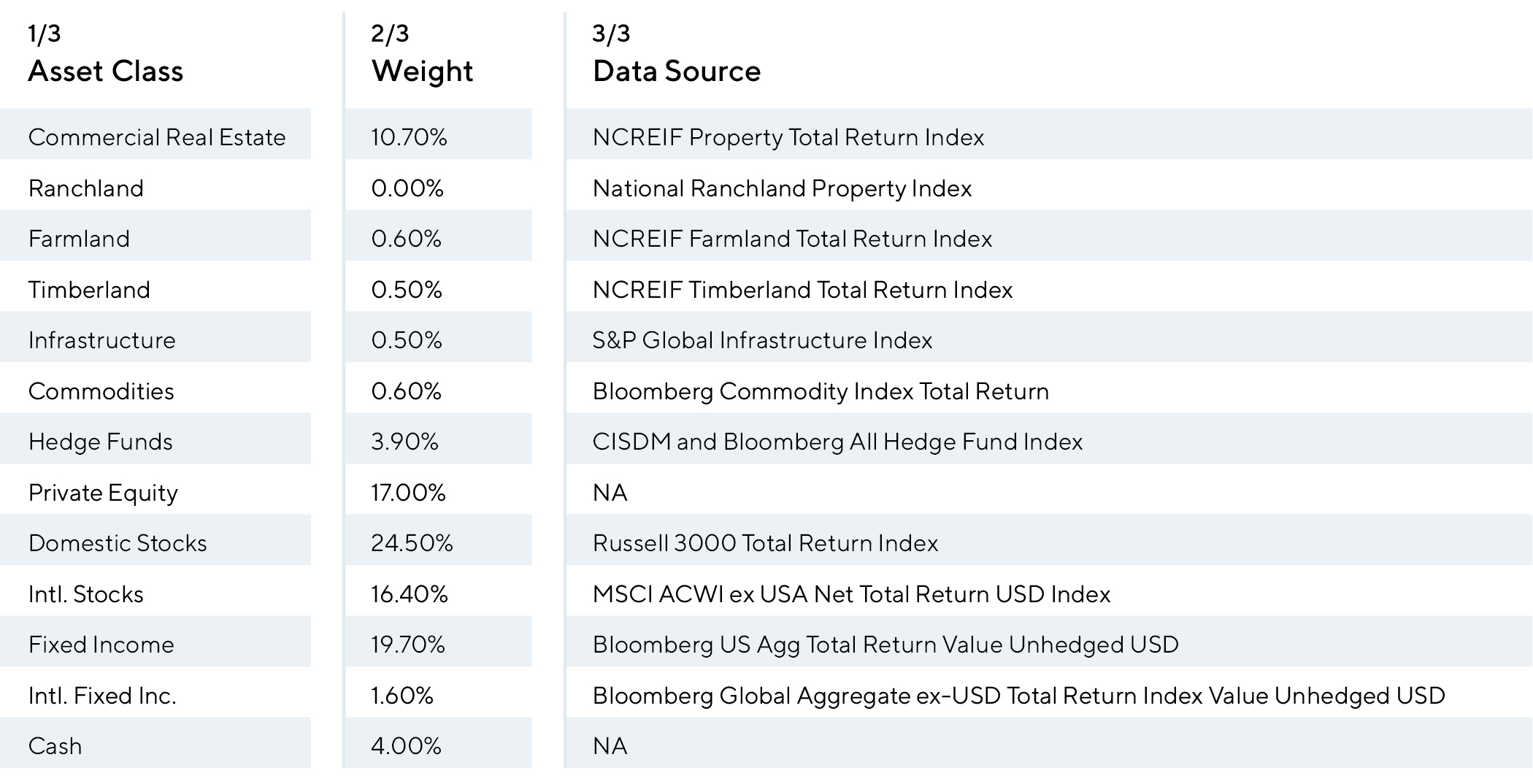
The historical performance of each asset class is charted in Figure 1 below:

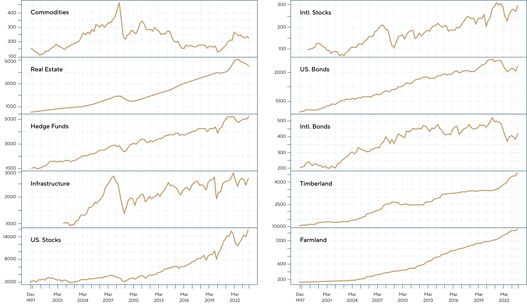
Most of these asset classes have generated positive returns over the past 25 years.  Based on this data, we performed a series of constrained portfolio risk/reward optimizations to find combinations of asset classes that could generate more efficient outcomes.

1.2. Optimization Method:

In order to find the optimal asset allocation mix, the following heavy-tail risk/reward optimization routine is used.

Let represent the discrete quarterly returns of the various asset classes described in section 1 above.

Step 1: Generate a random set of weights

Step 2: Calculate the hypothetical historical returns of the portfolio corresponding to this set of random weights, by calculating the matrix multiplication of weights and historical returns operation:

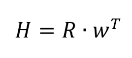
H represents the time series of the portfolio returns given the current portfolio weights.

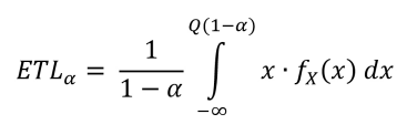
Step 3: Calculate the Expected Tail Loss of the portfolio based on the time series H, using the following heavy-tailed distribution:

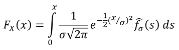
where  denotes the empirical density of the log-volatility of returns, estimated by kernel density estimation method.

Let denote the quantile function of the returns function, then the portfolio’s Expected Tail Loss (ETL) is given by:

We use the  as the measure of portfolio risk.

Steps 1 through 3 are repeated tens of thousands of times to generate the feasible portfolio universe.

Finally the best portfolio in terms of risk/reward is selected as the optimal allocation.

Because the system calculates the theoretical historical returns of the portfolio given a set of weights, there is no need for an explicit correlation assumption. In fact, using this method is superior from both a statistical and risk management point of view, in estimating what the current returns of the portfolio would be in an extreme market scenario. Indeed, making correlation assumption reduces the modeling of the co-movement of securities to one ‘average’ number, which is likely to be unreliable in the tails. Risk practitioners are well-aware of the drawbacks of relying on correlation modeling, as correlations will go to 1.0 during peaks of market volatility, markedly different from the ‘normal’ values. 

The method of computing portfolio historical returns does not reduce the co-movement of securities to a single number, and thus avoids this well-known drawback.

Paired with a robust heavy-tail model and a coherent measure of risk (ETL), this method of optimization is orders of magnitude more robust than standard Mean Variance Optimization methods.  For portfolios that include alternative investments, such as the Milliman allocation, this holds especially true given the widely studied non-normal distributions of most alternative asset classes.

1.3. Portfolio Constraints Used:

To identify the optimal asset mix while also recognizing possible limitations to large-scale allocation shifts within pension portfolios, we established constraints at both the overall allocation level and the within-asset class level for Real Assets.

Within the Real Assets portfolio, we established a floor allocation weighting for Commercial Real Estate at 50.0% of the overall Real Asset allocation.

Within the overall asset allocation, we limited the optimal weights to +/- 20.0% from the original weighting identified in the Milliman study as a subjective constraint to reflect common target weight bands for rebalancing and strategic asset allocation changes.

Private Equity was excluded from the analysis, with a simplifying assumption that the original 17.0% weighting remained fixed in the final allocation.  This was due to restrictions on data availability during the lookback period.

Cash was held at 4.0% as a simplifying assumption, given the goal of the paper was to identify optimal portfolios for risky asset classes.  The heavy tail optimization results do not need to consider that allocation to cash for accurate conclusions, so we excluded it from the optimizer.

2. Optimal Allocations:

To find the optimal global allocation, we use a two-step approach. In Step 1, we optimize the Real Asset allocation in isolation. In Step 2, we use the Step 1 optimized allocation as one asset class and find its optimal weights with respect to other asset classes to yield a new global allocation.

2.1. Optimal ‘Real Assets’ Composition

The Milliman study shows the typical allocation to Real Assets to be:

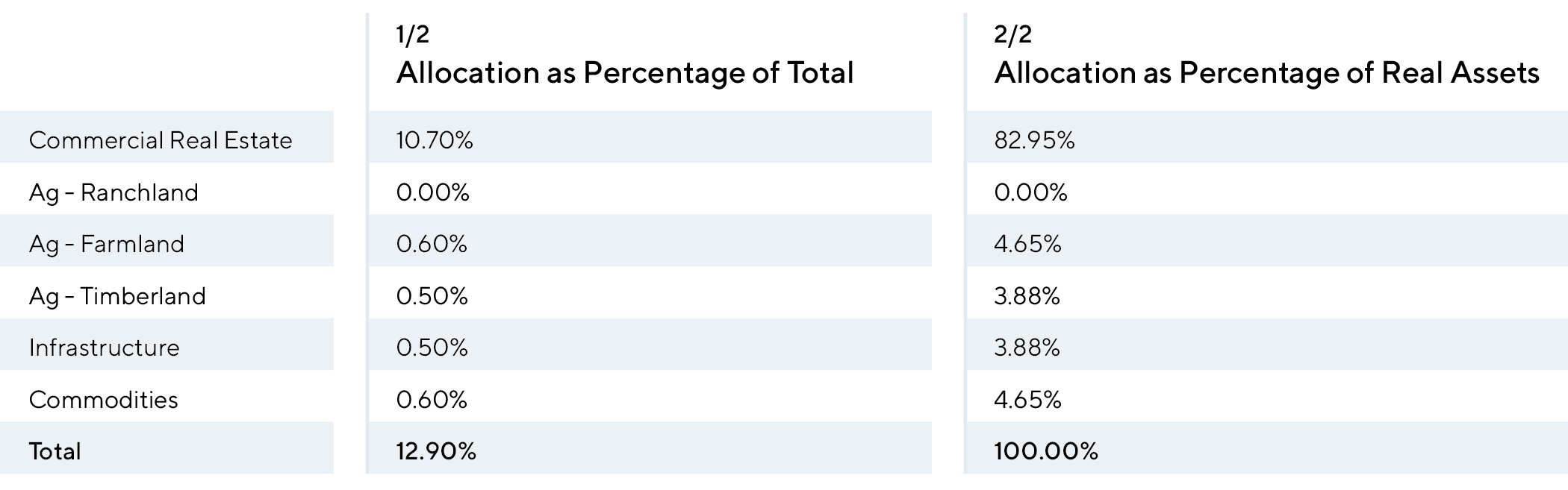
We repeat the optimization steps described in section 1.2 a total of 50,000 times with a constraint of no less than 50% of the current portfolio being allocated to Commercial Real Estate. While arbitrary, this limit reflects the reality that Commercial Real Estate investment opportunities are more widely available than other real asset classes and will likely be the dominant allocation for this very reason, among other restrictions such as liquidity needs.

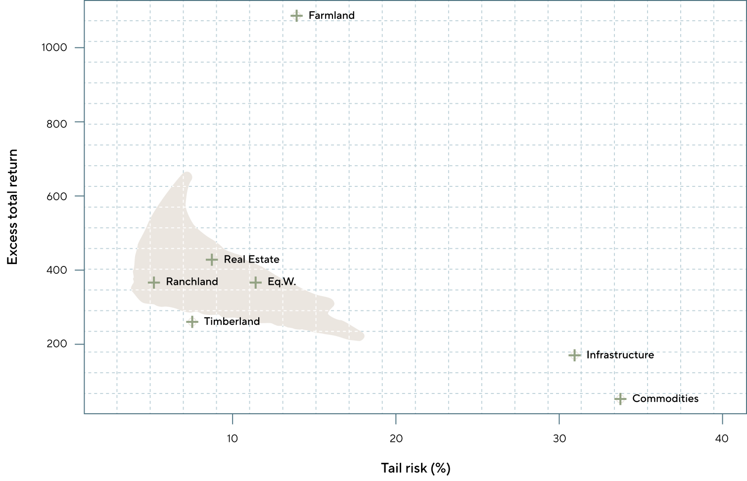
For each randomly generated set of weights, we plot the portfolios risk and reward. The X-axis represents the ETL(99%) of each portfolio combination, while the Y-axis represents the historical total return of the portfolio. More precisely, a reading of 500 means that an amount of $100 invested in the portfolio in 1998 would now be worth $500 more at the end of 2023.  

The feasible set is plotted in Figure 2 below. Farmland has the highest return of the lot, while Commodities have the lowest (as well as the highest tail risk). The “Eq.W” portfolio denotes the equally weighted portfolio.

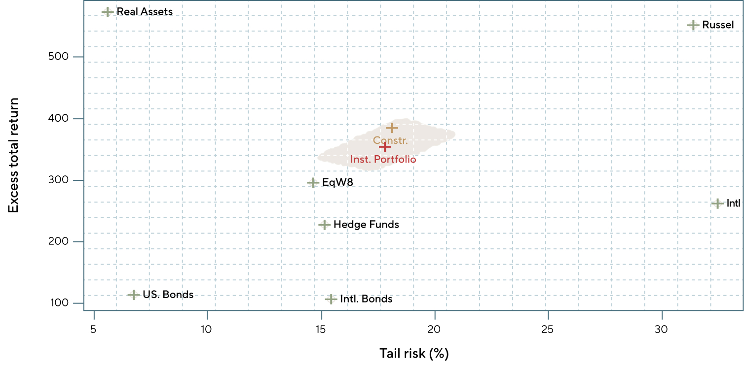
The optimal portfolio is selected by calculating the best risk/reward ratio in the neighborhood of the current institutional allocation, depicted in Figure 3 below:

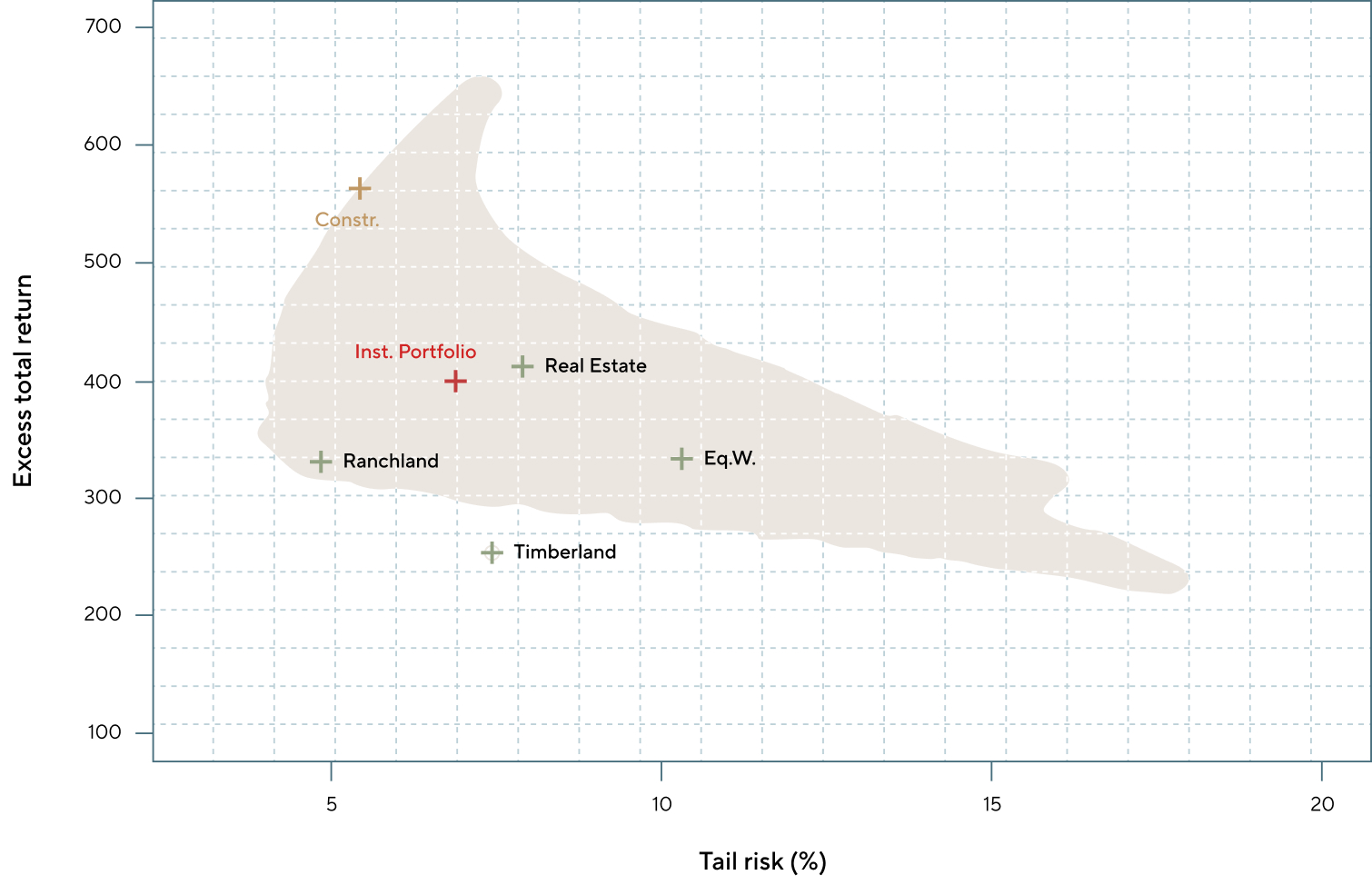
The constrained optimal portfolio (“Constr.”) is depicted in gold color, and lies on the efficient frontier. The current allocation described in the Milliman paper (“Inst. Portfolio”) is depicted in red. 

The most efficient mix of real assets is given in the table 3 below:

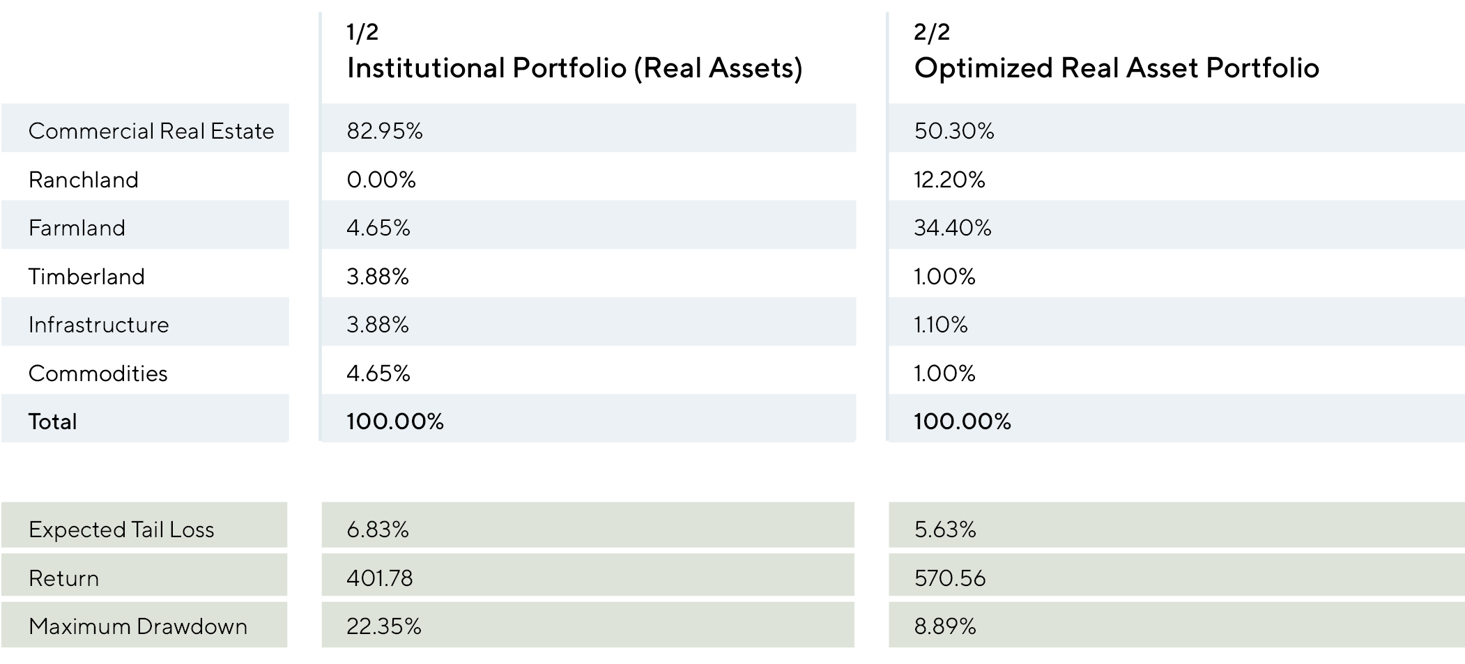
The Optimized portfolio results in a significant reduction of risk, measured by ETL (5.63% optimized vs 6.83% originally) and max drawdown (8.89 % vs 22.35%) while simultaneously benefitting from an increase of 42% in expected value (570.56 vs 401.78). The resulting optimized portfolio has lower allocations in Real Estate, Infrastructure and Timberland, and increased allocations in Farmland (34.4% vs 4.65%) and Ranchland (12.2%).

2.2. Optimal ‘Real Assets’ Allocation in the Overall Portfolio

With the optimized Real Asset portfolio, we now attempt to determine if a weight of 12.90% is indeed the best weight for Real Assets inside the global portfolio described in the Milliman study.

The same optimization procedure described in section 1.2 is repeated 200,000 times. We constrain portfolio weights to be within 20% of their current values, again to express the realities around liquidity and availability.

The feasible universe of portfolios is depicted in Figure 5 below:

The optimized portfolio is described in Table 4 below:

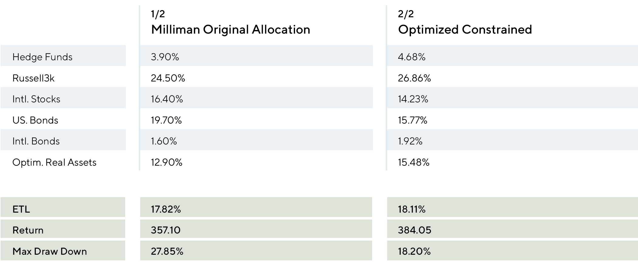
Even with relatively tight constraints, it is possible to find more efficient allocations of the global institutional portfolio, which results in an increase of over 7.5% in return with effectively no change in risk from current level.

2.3. Optimal Milliman Study Portfolio

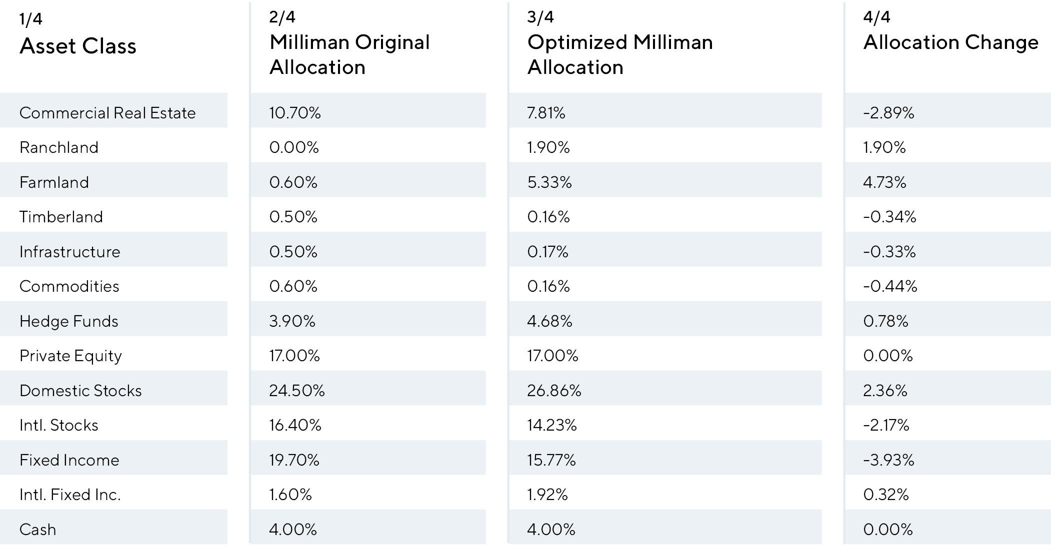
Applying the optimal weighting of Real Assets within the overall portfolio results in a final allocation summarized in table 5 below:

Conclusion:

In this paper we study the composition of the typical institutional allocation to Real Assets. We show that this bucket is typically too heavy in Commercial Real Estate, and would offer significantly better risk / reward characteristics by increasing the weighting of investments into other within-class options, namely Farmland and Ranchland. Moreover, it could be also argued that an increased allocation to Real Assets could benefit the efficiency of the typical institutional Portfolio when considering tail risk. 

The final optimized portfolio resulted in an increased weighting of 15.48% to Real Assets, leading to a decrease in both expected tail loss and maximum drawdown while improving excess returns.